Spectral Inputs

This package aims to provide a python interface to line-by-line calculations of absorption coefficients that is “traceable to benchmarks”. The overall goal is to treat lines, cross-sections, continua, collision-induced absorption, and line mixing. The package is structured so that the user can have multiple back-ends to choose from when running the calculation (see the API section of this documentation). Spectral input data is downloaded from the web and stored in a local sqlite3 database, which we expect the users to build (or rebuild) before running any calculations using a simple API consisting of a Database and HitranWebApi object.

Creating the local spectral database

To create the spectral database, start by creating HitranWebApi and Database objects:

from pyLBL import Database, HitranWebApi
webapi = HitranWebApi("<your HITRAN API key>")  # Prepare connection to the data sources.
database = Database("<path to database>")  # Make a connection to the database.
database.create(webapi)  # Note that this step will take some time.

Line data will be downloaded from HITRAN. Your HITRAN API key is a unique string provided to each account holder by the HITRAN website. You must make an account there. In order to get your api key, create an account, log in, click on the little person icon near the top right part of the screen to get to your profile page (or navigate to profile) and copy the long string listed as your “API Key”. Note that keeping track of which version of the HITRAN data that is being downloaded is still currenlty under development.

For treatment of molecular continua, we use a python port of MT-CKD developed by AER. Currently, the python port is based on version 3.5 and reads data from an automatically downloaded netCDF dataset. This dataset includes the effects of collision-induced absorption. In the near future it is expected that this data will be incorporated into the HITRAN database and once it is this package will be updated to instead download it from there.

For treatment of cross-sections (polynomial interpolation in temperature and/or pressure), we use a model developed at the University of Hamburg (UHH). This model provides data in netCDF datasets, which are downloaded automatically.

Downloading the data and creating the database only needs to be done at least once, can take a significant amount of time (~30 minutes).

Re-using an existing spectral database

Once a local spectral database is created, it can be re-used by simply connecting to it:

from pyLBL import Database
database = Database("<path to database>")

Since the database already exists and is populated, there is no longer a need to create a HitranWebApi object.

Defining the spectral grid

Spectral grid input should in wavenumber [cm-1] and be defined as a numpy array, for example:

from numpy import arange
grid = arange(1., 5001., 0.1)

Also as of now, the wavenumber grid resolution should be one divided by an integer. This requirement may be relaxed in the future.

Spectral database schema

The local spectral database uses sqlite3 and consists of a series of tables.

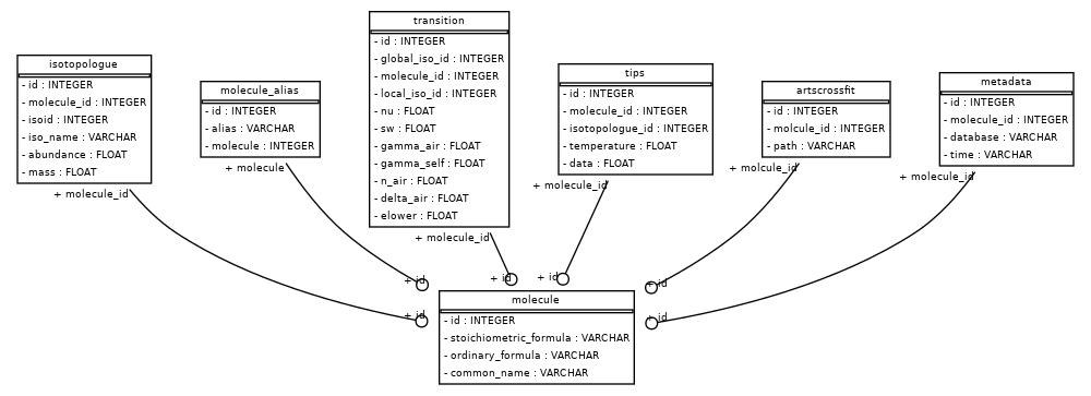
The molecule table stores all the unique molecules found in the HITRAN database. It links to all of the other tables through each molecules’s unique id. In order to improve accessibility, each molecule can have associated string aliases which are stored in the molecule_alias table. For example, “H2O”, “water vapor”, etc. are all aliases for H2O, and can be used to find H2O in the database. Each molecule may have many different forms known as istolopologues. These isotopologues are stored in the isotopologue table, and have their own ids, names, masses, and abundance amounts. Each isotopologue contains many molecular lines, or transitions between quantum states. The properties of these transitions are downloaded from HITRAN and stored in the transition table. Furthermore, each isotopologue has a table of total internal partition functions values at various temperatures which are stored in the tips table. For some molecules, explicit molecular lines are not treated directly, but absorption cross-sections are instead calculted using polynomial interpolation in temperature and/or pressure). Paths to the datasets that store these cross-section tables are stored in artscrossfit table.